|
|
As a young academic I spent my days on computational statistical thermodynamics. That is quite a mouthful, so let me explain. Some years ago I wrote an introduction to classical thermodynamics explaining that this theory on bulk matter is not concerned with the structure of matter. It works fine for steam engines or submarines, but is not satisfactory when describing processes at a very small scale. For that, we have statistical thermodynamics. Brilliant minds like Maxwell, Boltzmann and Liouville devised the framework for this theory. In a nutshell, statistical thermodynamics explains the likelihood of tiny particles being in a certain configuration, and that the value of a bulk property is the average of that property in all attainable configurations, weighed by their likelihood.
All we would have to do is derive exact equations to compute all there is to know about gaseous, liquid or solid matter. Alas, more times than not solving these equations on paper is mathematically impossible. In computational statistical thermodynamics we numerically calculate the results of these unsolvable equations. The idea is to observe a (large) number of particles, following their movement for a while, and averaging properties as we go along. Two common methods to this end are Molecular dynamics or Monte Carlo simulations. Sometimes these methods are referred to as "computational microscopes". Instead of a mathematical formula, you get a table with numbers. Theorists use the tables to develop their math, and engineers use them for their jobs.
Monte Carlo was the first technique I used, for my graduation study. Put simply, the idea behind Monte Carlo simulations in statistical thermodynamics is as follows. You set up particles in some suitable initial configuration, that has a likelihood of existing as predicted by theory. Then you modify it, for instance by moving a particle a bit, or swapping two of them, or resizing the entire system. That yields a new configuration with its own likelihood of existing. Now you roll dice to decide whether to accept the new configuration as the new one or revert to the old one, depending on the configurational likelihoods. Repeat these modifications many times, and you will eventually generate the most likely configurations for your set of particles. Average what you want to know in these configurations, and you arrive at a good approximation of the theoretical results.
My graduation supervisor at the University of Nijmegen, a sharp-minded theoretical physicist, offered me a graduation subject in which I would write from scratch a Monte Carlo program and with that study the thermodynamics of solid-liquid interfaces. The results of such studies relate to for instance industrial crystal growth, which makes the subject technically relevant. The task sounded like music to my ears - I would be a heavy user of the university computer centre, and as a chemist I would work with theoretical physicists. It was a bit odd though that in the Nijmegen chemistry department only subjects in molecular quantum mechanics were understood as "theoretical chemistry".
I have all this time kept a copy of the source code of abovementioned program, which proved an excellent test case for my own Fortran compiler. It turned out that my revived Monte Carlo program worked beautifully. As expected, compared to the mainframe it ran on in the 1980's, performance has much improved. In an hour, I can do what took weeks in the 1980's, not only because of improved processing speed, but also because I do no need to share capacity anymore. At the time, heavy jobs ran in batch outside office hours, and I had to queue with my colleagues from theoretical chemistry, crystallography, high energy physics, astrophysics, etcetera.
Of course I could not resist revisiting some of the research I did at the time just for the fun of it, with the benefit of modern ray-tracing software to draw compelling images of the particle configurations. Here I want to showcase a few observations for a mixture of xenon and neon at very low temperature. Noble gases are popular models in simulations since interactions between atoms are quite well understood and relatively simple. Very briefly, this is how two noble gas atoms interact - they push at short distance, pull at intermediate distance but essentially ignore each other at long distance, while a nearby third atom does not influence the interaction between the two.
I performed the simulations as if we were still in the 1980's and considered an amount of atoms that would have been just about feasible at the time, if I would have had access to the supercomputers of the era. Hence we consider a bit over 10,000 xenon atoms and the same number of neon atoms, in a rectangular box. On our university's mainframe, feasible atom count was about an order of magnitude lower. To model a bulk system, the rectangular box containing the atoms is periodically continued in all three dimensions. Periodic boundary conditions give rise to finite size effects, any good simulation study addresses those.
In the real world, most experiments in a laboratory are done at constant pressure. We will do something comparable in our simulations, and compare simulations at different temperatures but at a same pressure. You will appreciate that particle interactions contribute to the pressure - the pushing and pulling between atoms causes physical stress. One approach is to make the particles "stress free", that is to resize volume such that contributions to the pressure from particle interactions cancel on average. This means that we direct the pressure in the simulations towards the ideal gas pressure.
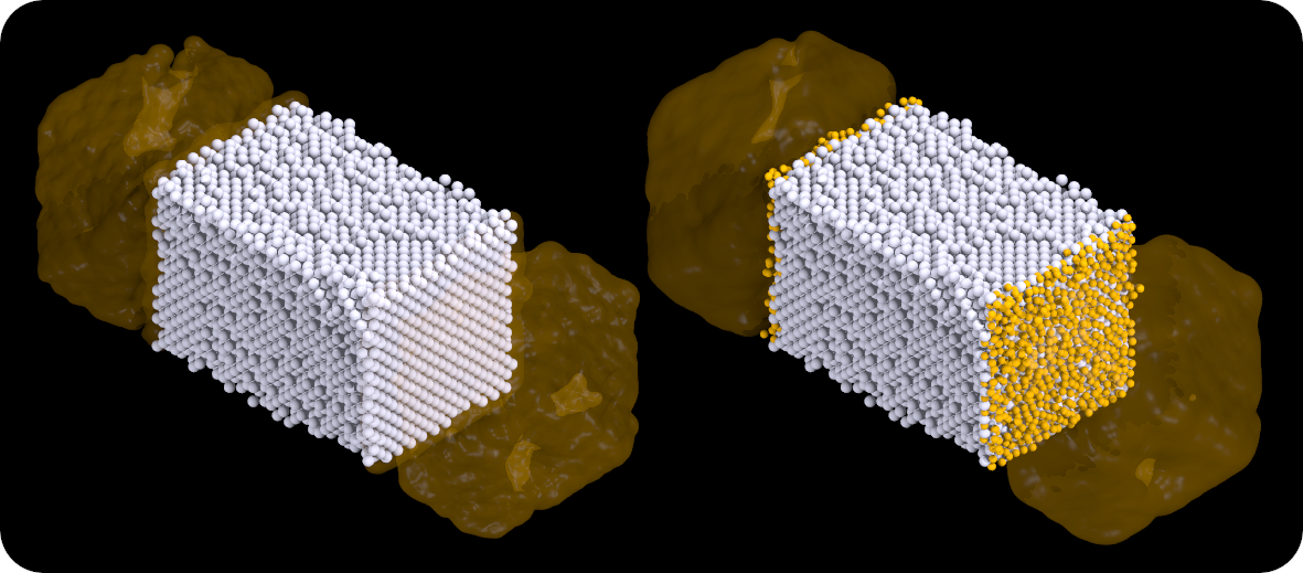
Our first run is at a temperature of 25K, which is the melting point of neon. Below is a snapshot of the box - white spheres are xenon atoms and orange spheres are neon atoms. Molten neon is drawn as a blob for clarity. No xenon atoms dissolve in the neon liquid yet. Xenon melts at 161K, and to the left we see that xenon is indeed solid with a flat crystal surface. To the right is the same configuration showing the neon atoms bordering the crystal surface. Note that these atoms seem frozen onto the xenon crystal - a liquid close to an interface apparently assumes structure. For a particle to behave in a "liquid" manner, it must be free to move in any direction. Near a solid wall, that freedom is limited.

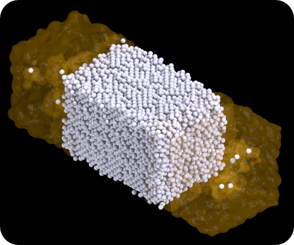
A snapshot configuration at 120K is shown below. Now we do see some xenon atoms that have dissolved in the neon liquid. We also observe that the crystal surface is no longer flat. A more in-depth analysis of these simulations shows that indeed the outer layers of a crystal melt at a lower temperature than the melting point of the bulk crystal. This was a cool discovery from my simulation work at the time, since coincidentally "surface melting" was demonstrated experimentally on real lead crystals at AMOLF. Our model is less complex than a lead surface, still we observed the same phenomenon in our simulations.

After graduation I was offered a position at the applied physics faculty at the University of Twente, where I again worked with theoretical physicists, always hungry for computational resources. A bright guy followed up on my simulation work in Nijmegen, and eventually an article¹ was published. After academia, my career moved away from intensive computation, only to return there in recent years thanks to the rise of industrial application of machine learning and artificial intelligence. However, reviving forty-year old source code brought back many good memories of my first substantial programming and research work.
¹ J.P. van der Eerden, A. Roos, J.M. van der Veer. Surface roughening versus surface melting on Lennard-Jones crystal surfaces. Journal of Crystal Growth 99(1–4) 77-82 [1990].
|
© 2002-2026 J.M. van der Veer (jmvdveer@xs4all.nl)
|